Installing OTBTF from sources can take some time, between preparing the system with prerequisites, and waiting that the compiler finish to build the two giants Orfeo ToolBox and TensorFlow. In addition, if you compile TensorFlow with CUDA, it can takes several hours! Regarding this matter, I started to make some docker images to ease the deployment of OTBTF. With the incoming release of OTB-7.0, I had to make some updates in the OTBTF build, and decided to look how to make a container that is able to use GPU.
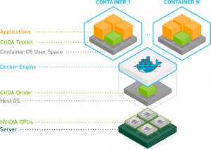
The NVIDIA runtime
NVIDIA have developed some convenient abstraction layer for using NVIDIA GPUs on docker. It handles cuda/gpu drivers of the host system, enabling its use inside the docker containers that runs on top of it.
First, you have to install your GPU drivers and CUDA. All the installers are available on NVIDIA website. In my case, I did that with the 430.50 driver for the GTX1080Ti and CUDA 10.1.
After everything is installed, you will need to reboot your machine. Then check that the nvidia-persistenced service is running.
cresson@cin-mo-gpu:~$ systemctl status nvidia-persistenced.service
● nvidia-persistenced.service – NVIDIA Persistence Daemon
Loaded: loaded (/lib/systemd/system/nvidia-persistenced.service; static; vendor preset: enabled)
Active: active (running) since Fri 2019-10-11 15:08:40 UTC; 3 days ago
Process: 1296 ExecStart=/usr/bin/nvidia-persistenced –user nvidia-persistenced –no-persistence-mode –verbose (code=exited, status=0/SUCCESS)
Main PID: 1321 (nvidia-persiste)
Tasks: 1 (limit: 4915)
CGroup: /system.slice/nvidia-persistenced.service
└─1321 /usr/bin/nvidia-persistenced –user nvidia-persistenced –no-persistence-mode –verbose
You can also check that you GPUs are up using nvidia-smi:
+—————————————————————————–+ | Processes: GPU Memory | | GPU PID Type Process name Usage | |=============================================================================| | No running processes found | +—————————————————————————–+
Run the OTBTF docker image with NVIDIA runtime enabled. You can add the right permissions to you current USER for docker (there is a “docker” group), or you can also use root to run a docker command . The following command will display the help of the TensorflowModelServe OTB application.
docker run –runtime=nvidia mdl4eo/otbtf1.7:gpu otbcli_TensorflowModelServe -help
And that’s all! Now the mdl4eo/otbtf1.7:gpu docker image will be pulled from DockerHub and available from docker. Don’t forget to use th NVIDIA runtime (using –runtime=nvidia) else you won’t have the GPU support enabled.
Here is what happening when docker pulls the image (i.e. first use, after the pull is finished):
The different stages are download from DockerHub (You can retrieve them from the dockerfiles provided on the OTBTF repository). When your command prompt prefix is “root@039085b63ea3“, you are inside the running docker container as root!
And then… how to use Docker?
Well, I do not intend to make a full tutorial about docker here 😉 In addition, I am far from being an expert in this area.
But here are a few stuff I used to make things work with docker. I don’t think at all that it is good practice, but these tips can help.
Docker run
The previous command showed you how to enter a container in interactive mode. From here, you can install new packages, create new users, run applications, etc.
Docker commit
Docker is like git. When you enter a docker container, you can modify it (e.g. install new packages) and commit your changes. If you don’t, every changes you made inside the container are erased when you leave the container (i.e. “exit” it).
Do a few changes in your running container, like installing a new package. Then, use another terminal to commit your changes:
Here, 3ade7b0dc71b comes from the first terminal in which your container is running. You can copy/paste the hash from the command prompt prefix (“root@3ade7b0dc71b“).
Mount some filesystem
And now you want to do some deep learning experiments on your favorite geospatial data… How to mount some persistent filesystem in your docker container?
There is useful options in the docker run command, like -v /host/path/to/mount:/path/inside/dockercontainer/ which will mount the host directory /host/path/to/mount inside your docker container as the /path/inside/dockercontainer/ path.
cresson@cin-mo-gpu:~$ sudo docker run –runtime=nvidia -ti -v /home/cresson/:/home/toto mdl4eo/otbtf1.7:gpu bash
root@e4a2b1c649c9:/# touch /home/toto/test
root@e4a2b1c649c9:/# exit
exit
cresson@cin-mo-gpu:~$ ls /home/cresson/test
/home/cresson/test
You will have to grant the right permissions to the mounted directory, particularly once you will add some non-root users inside your docker container.
For instance, if you have a user “otbuser” inside your docker container, you can do the following:
Check the file permissions of your host shared volume (note the GID of the volume)
Create a new group “newgroup” which has the same GID of the volume you want to use
There is various kind of remote sensing images: drone, aerial, satellite, multi-temporal, multi-spectral, … and each product has its advantages and weaknesses. What if we could synthesize a “super-resolution” sensor that could benefit from the advantages of all these image sources? For instance, what if we could fuse (1) high spatial resolution sensor (you know, the one that passes 1 time a year over your ROI), and (2) high temporal resolution sensor (…of which images can’t even let you identify where’s your house!) to derive one synthetic super sensor that has high spatial and high temporal resolution?
Today’s data-driven deep learning techniques establish state of the art results that would be crazy not to consider.
Super-resolution Generative Adversarial Networks
In their paper (“Photo-Realistic Single Image Super-Resolution Using a Generative Adversarial Network“, which is quite a good read), Ledig et al. propose an approach to enhance low resolution images. They use Generative Adversarial Networks (GAN) to upsample and enhance a single low resolution image, such as the result is looking as the target (high resolution) image. GANs consist in two networks: the generator and the discriminator. In one hand, the generator transforms the input image (the low-res one) into an output image (the synthesized high-res one). In the other hand, the discriminator inputs two images (one low-res image, and one high-res image), and produce a signal that expresses the probability that the second image (the high-res) is a real one. The objective of the discriminator is to detect “fake” (i.e. synthesized) hi-res images among real ones. Simultaneously, the objective of the generator is to produce good looking hi-res images that fool the discriminator, and that are also close to the real hi-res images.
From images to remote sensing images
Now suppose we have some high res remote sensing images (say Spot 6/7, with 1.5m pixel spacing) and some low res remote sensing images (like Sentinel-2, with 10m pixel spacing) and we want to enhance the low res images at the same resolution of the high res. We can train our SRGAN generator over some patches and (try to…) make Sentinel-2 images look like Spot 6/7 images !
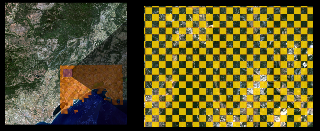
First I have downloaded a Sentinel-2 image from the Theia data center. The image is a monthly synthesis of multiple Sentinel-2 surface reflectance scenes produced with MAJA software (see here for details). The image is cloudless, thank to the amazing work of the CNES and CESBIO guys. I used a pansharpened Spot 6/7 scene acquired in the same month as the Sentinel-2 image, in the framework of the GEOSUD project.
The tools of choice to perform this are the OrfeoToolbox with OTBTF (a remote module that uses TensorFlow). First, we extract some patches in images (using otbcli_PatchesExtraction).
About 6k patches are sampled in images.
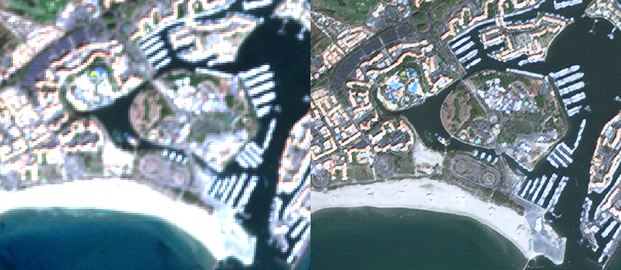
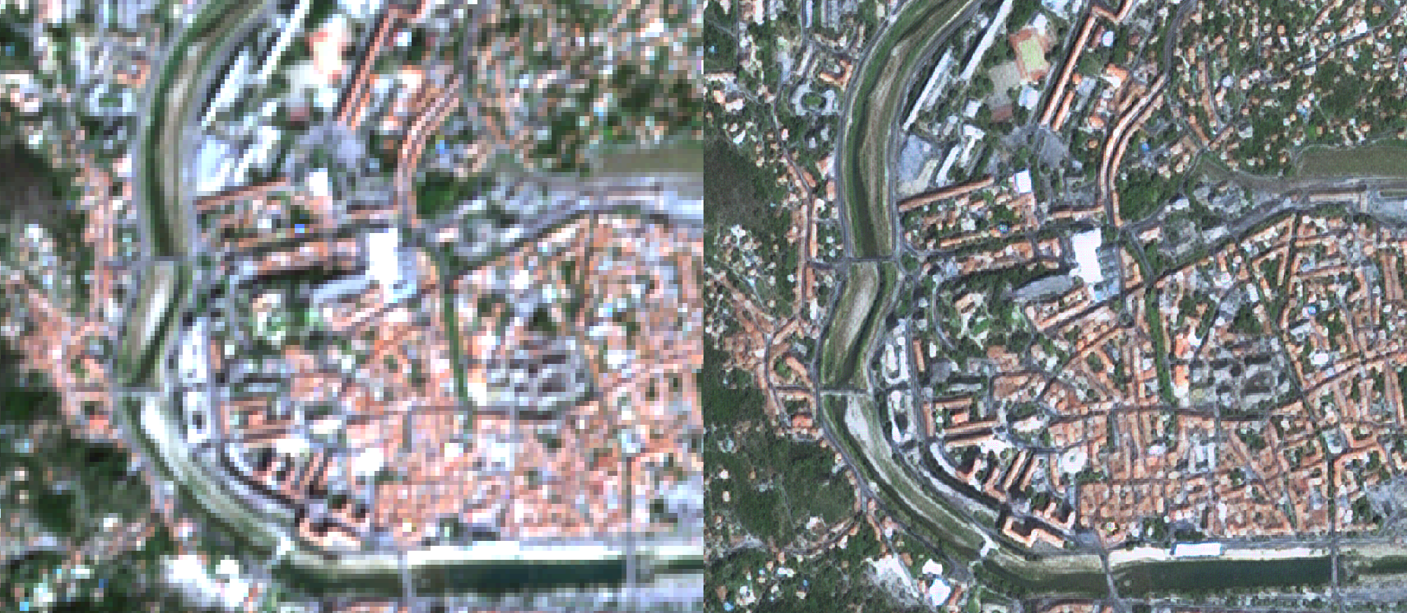
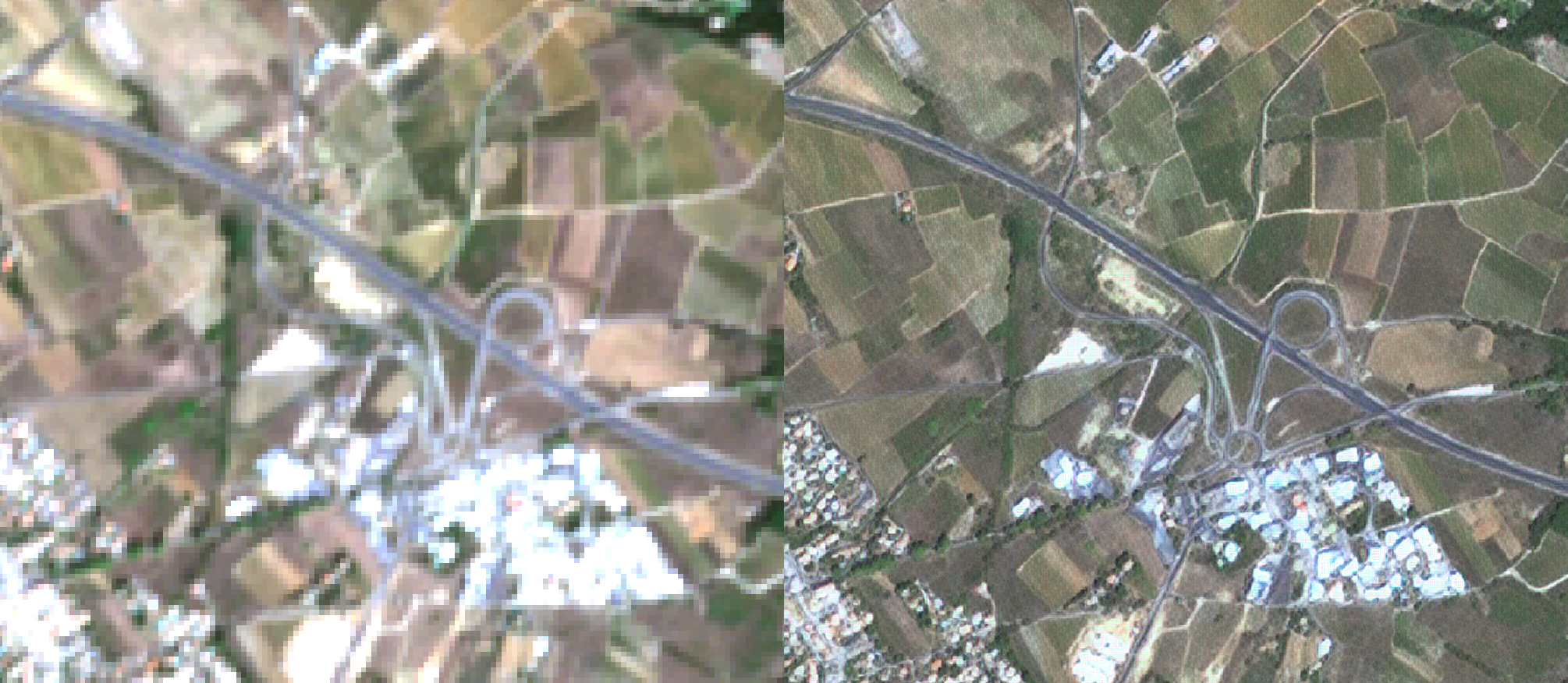
Once this is done, we can train our generator over these patches, using some SRGAN-inspired code (since we can find many SRGAN implementations on github!). After the model is trained properly, we can transform our Sentinel-2 scenes into images with 1.5m pixel spacing using the otbcli_TensorflowModelServe application (first time that I had to set a outputs.spcscale parameter lower than 1.0!). The synthesized high resolution Sentinel-2 image has a size of 72k by 72k.
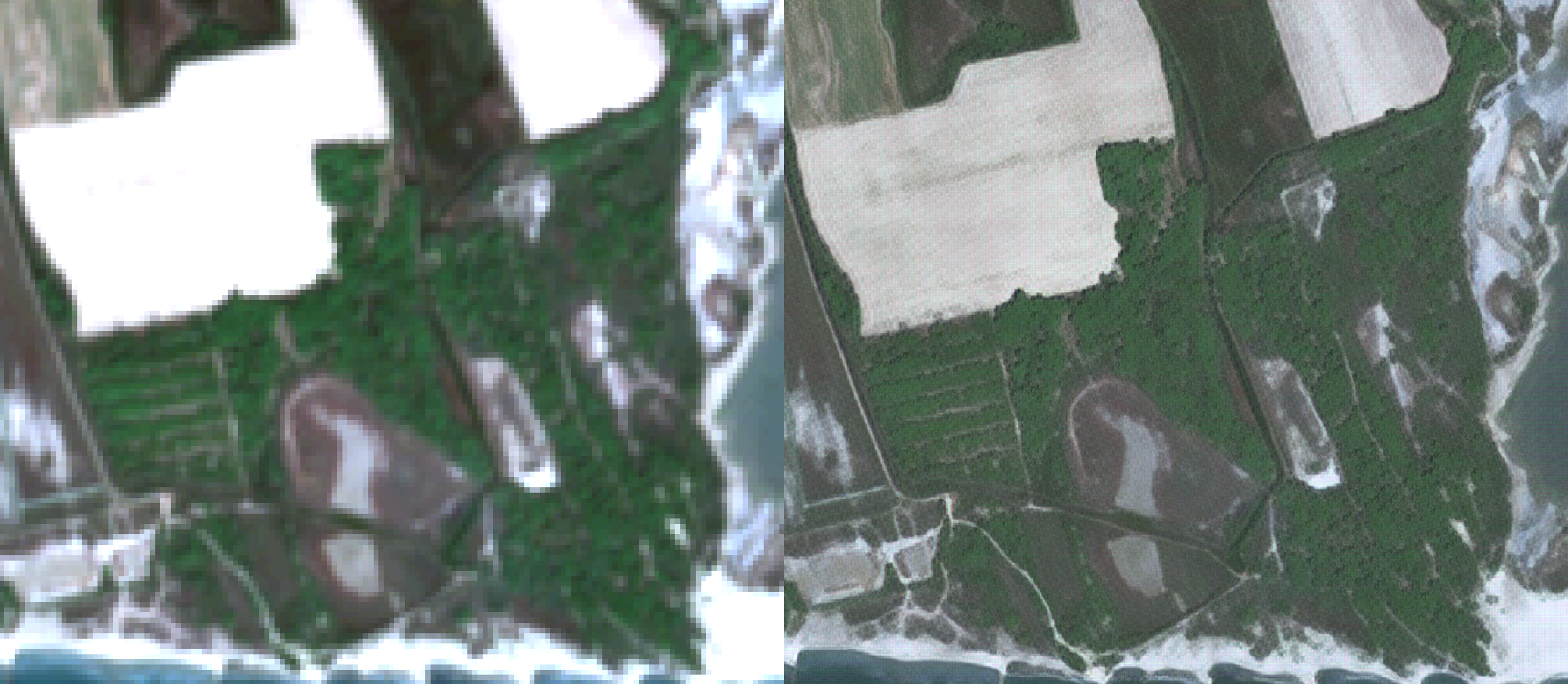
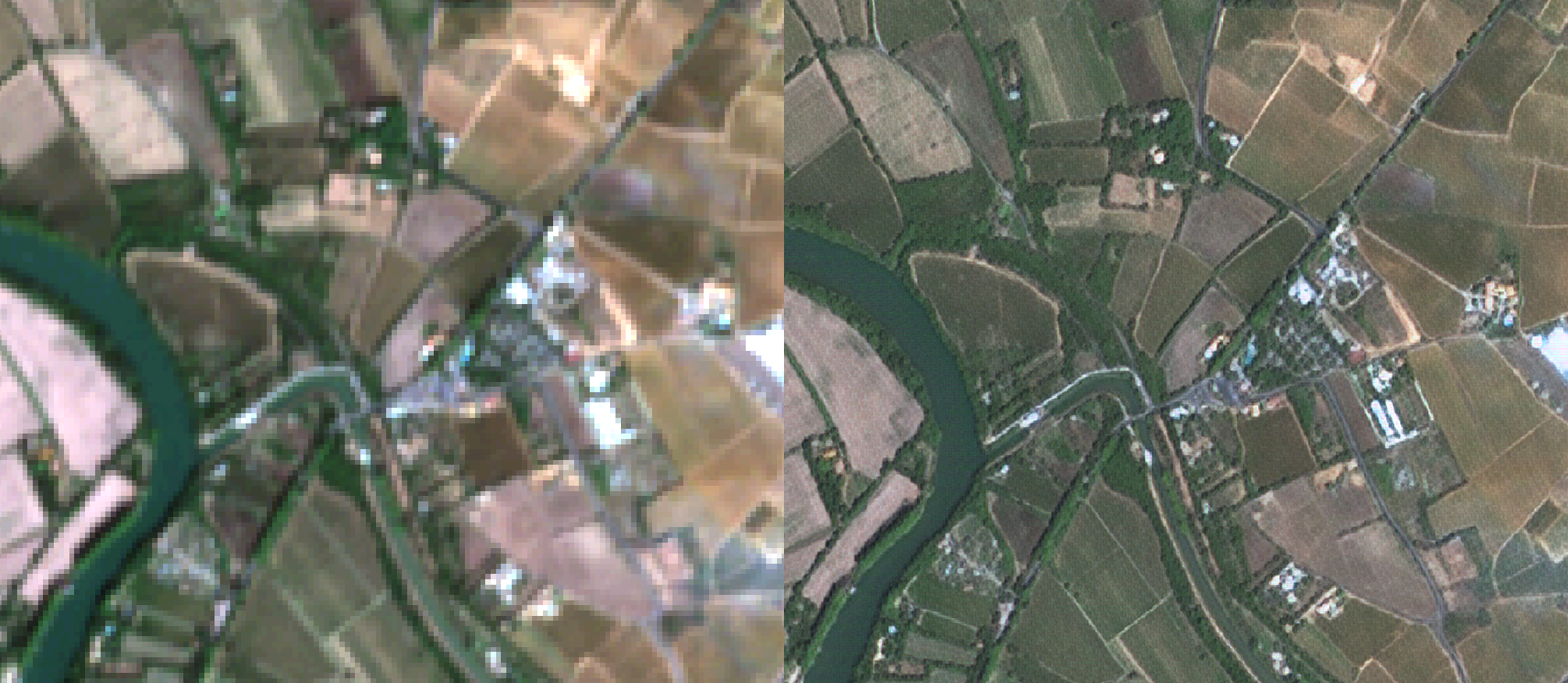
Below are a couple of illustrations. Left: the original RGB Sentinel-2 image, Right: the enhanced RGB Sentinel-2 image. In a sake of sincerity, we put images that are far away from learning patches. You can enlarge them to full resolution.
Full map
We put the entire generated image in a cartographic server. You can browse the map freely (Select the “S2_RGB (High-Res)” from the layer menu, to display the 1.5m Sentinel-2 image). You can also display patches used for training (“Training patches footprint” layer).
In this post we show what deep learning could offer in therm of data driven image enhancement for remote sensing images, at least for illustrative use.
Code
The code is available on Github. Feel free to open a PR to add your own model, or training loss, etc. !
Update (28/01/2020): open dataset, available for download!
In this tutorial, we will see how to train and apply a deep neural network on real world remote sensing images, using only user-oriented open-source software. No coding skills required!
Data
Our “Tokyo dataset” is freely available. It is composed as follow:
One Sentinel-2 image, that can be downloaded from the European Space Agency hub or from your preferred Sentinel access portal. Just download the Sentinel-2 image acquired over the city of Tokyo the 2019/05/08 (Mission: Sentinel-2, Platform: S2A_*) named S2A_MSIL2A_20190508T012701_N0212_R074_T54SUE_20190518T165701.
Two label images of terrain truth (one for training and one for validation). Each pixel is either a “no-data” value (255) or a class value (starting from 0). The files can be downloaded here (also provided: the style .qml file for QGIS). This dataset has been elaborated for educational purpose at our research facility, using Open Street Map data.
Goal
We want to classify the Sentinel-2 image, meaning that we intend to estimate the class for each pixel. Since our terrain truth data is sparsely annotated, our approach consist in training a network that estimates one single class value for a particular patch of image. If we had a densely annotated dataset, we could have used the semantic segmentation approach, but this will be another story (soon on this blog!).
We will use the OTBTF remote module of the Orfeo ToolBox. OTBTF relies on TensorFlow to perform numeric computations. You can read more about OTBTF on the blog post here.
OTBTF = Orfeo ToolBox (OTB) + TensorFlow (TF)
It is completely user-oriented, and you can use the provided applications in graphical user interface as any Orfeo ToolBox applications. Concepts introduced in OTBTF are presented in [1]. The easiest way to install and begin with OTBTF is to use the provided docker images.
Deep learning backgrounds
To goal of this post is not to do a lecture about how deep learning works, but quickly summarizing the principle!
Deep learning refers to artificial neural networks with deep neuronal layers (i.e. a lot of layers !). Artificial neurons and edges typically have parameters that adjust as learning proceeds.
Weights modify the strength of the signal at a connection. Artificial neurons may output in non linear functions to break the linearity, for instance to make the signal sent only if the aggregate signal crosses a given threshold. Typically, artificial neurons are aggregated into layers. Different layers may perform different kinds of transformations on their inputs. Signals travel from the first layer (the input layer), to the last layer (the output layer), possibly after traversing the layers multiple times. Among common networks, Convolutional Neural Networks (CNN) achieve state of the art results on images. CNN are designed to extract features, enabling image recognition, object detection, semantic segmentation. A good review of deep learning techniques applied to remote sensing can be found here [2]. In this tutorial, we focus only on CNN for a sake of simplicity.
Let’s start
During the following steps, we advise you to use QGIS to check generated geospatial data. Note that applications parameters are provided in the form of command line, but can be performed using the graphical user interface of OTB!
We can decompose the steps that we will perform as follow:
Sampling: we extract patches of images associated to the terrain truth,
Training: we train the model from patches,
Inference: Apply the model to the full image, to generate a nice landcover map!
Normalize the remote sensing images
We will stack and normalize the Sentinel-2 images using BandMathX. We normalize the images such as the pixels values are within the [0,1] interval.
# Go in S2 folder cd S2A_MSIL2A_20190508T012701_N0212_R074_T54SUE_20190508T041235.SAFE cd GRANULE/L2A_T54SUE_A020234_20190508T012659/IMG_DATA/R10m/
The first step to apply deep learning techniques to real world datasets is sampling. The existing framework of OTB offers great tools for pixel wise or object oriented classification/regression tasks. On the deep learning side, nets like CNNs are trained over patches of images rather than batches of single pixel. Hence the first application of OTBTF we will present targets the patches sampling and is called PatchesExtraction.
The PatchesExtraction application integrates seamlessly in the existing sampling framework of OTB. Typically, we have two options depending if our terrain truth is vector data or label image.
Vector data: one can use the PolygoncClassStatistics (computes some statistics of the input terrain truth) and SampleSelection applications to select patches locations, then give them to the PatchesExtraction application.
Label image: we can directly use the LabelImageSampleSelection application from the OTBTF to select the patches locations.
In our case, we have terrain truth in the form of a label image. We hence will use option 2. Let’s select 500 samples for each classes with the command line below:
# Samples selection for group A
otbcli_LabelImageSampleSelection \
-inref ~/tokyo/terrain_truth/terrain_truth_epsg32654_A.tif \
-nodata 255 \
-outvec terrain_truth_epsg32654_A_pos.shp \
-strategy "constant" \
-strategy.constant.nb 500
Where :
inref is the label image,
nodata is the value for “no-data” (i.e. no annotation available at this location),
strategy is the strategy to select the samples locations,
outvec is the filename for the generated output vector data containing the samples locations.
Repeat the previously described steps for the second label image (terrain_truth_epsg32654_B.tif). Open the data in QGIS to check that the samples locations are correctly generated.
Patches extraction
Now we should have two vector layers:
terrain_truth_epsg32654_A_pos.shp
terrain_truth_epsg32654_B_pos.shp
It’s time to use the PatchesExtraction application. The following operation consists in extracting patches in the input image, at each location of the terrain_truth_epsg32654_A_pos.shp. In order to train a small CNN later, we will create a set of patches of dimension 16×16 associated to the corresponding label given from the class field of the vector data. Let’s do this :
source1 is first image source (it’s a parameter group),
source1.il is the input image list of the first source,
source1.patchsizex is the patch width of the first source,
source1.patchsizey is the patch height of the first source,
source1.out is the output patches image of the first source,
vec is the input vector data of the points (samples locations),
field is the attribute that we will use as the label value (i.e. the class),
outlabels is the output image for the labels (we can force the pixel encoding to be 8 bits because we just need to encore small positive integers).
After this step, you should have generated the following output images, that we will name “the training dataset”:
Sentinel-2_B4328_10m_patches_A.tif
Sentinel-2_B4328_10m_labels_A.tif
Trick to check the extracted patches from QGIS : Simply open the patches as raster layer, then chose the same coordinates reference system as the current project (indicated on the bottom right of the window).
Repeat the previously described steps for the vector layer terrain_truth_epsg32654_B_pos.shp and generate the patches and labels for validation. After this step, you should have the following data that we will name “the validation dataset” :
Sentinel-2_B4328_10m_patches_B.tif
Sentinel-2_B4328_10m_labels_B.tif
Side note on pixel interleave: sampled patches are stored in one single big image that stacks all patches in rows. There is multiple advantages to this. In particular, accessing one unique big file is more efficient than working on thousands of separate small files stored in the file system. The interleave of the sampled source is also preserved, which, guarantee good performance during data access.
Training
How to train a deep net ? To begin with something easy, we will train a small existing model. We focus on a CNN that inputs our 16 × 16 × 4 patches and produce the prediction of an output class among 6 labels ranging from 0 to 5.
Basics
Here is a quick overview of some basic concepts about the training of deep learning models.
Model training usually involves a gradient descent (in the network weights space) of a loss function that typically expresses the gap between estimated and reference data. The batch size defines the number of samples that will be propagated through the network for this gradient descent. Supposing we have N training samples and we want to use a batch size of n. During learning, the first n samples (from 1 to n) will be used to train the network. Then, the second n samples (from n+1 to 2n) will be used to train the network again. This procedure is repeated until all samples are propagated through the network (this is called one epoch).
Model guts
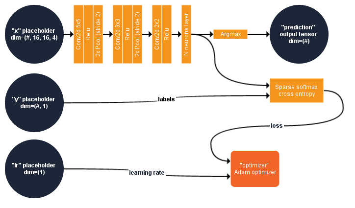
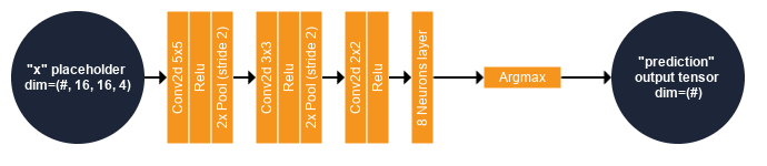
We propose to introduce a small and simple CNN to better understand the approach. This section describe what is inside this model. The figure below summarizes the computational graph of our CNN.
Input : The image patches fed the placeholder named “x” in the TensorFlow model. The first dimension of “x” might have any number of components. This dimension is usually employed for the batch size, and isn’t fixed to enable the use of different batch size. For instance, assuming we want to train our model with a batch of 10 samples, we will fed the model a multidimensional array of size 10 × 16 × 16 × 4 in the placeholder “x” of size # × 16 × 16 × 4.
Deep net : “x” is then processed by a succession of 2D-Convolution/Activation function (Rectified linear)/Pooling layer. After the last activation function, the features are processed by a fully connected layer of 6 neurons (one for each predicted class).
Predicted class : The predicted class is the index of the neuron (from the last neuron layer) that output the maximum value. This is performed in processing the outputs of the last fully connected layer with the Argmax operator, which is named “prediction” in the graph.
Cost function : The goal of the training is to minimize the cross-entropy between the data distribution (real labels) and the model distribution (estimated labels). We use the cross-entropy of the softmax of the 6 neurons as a cost function. In short, this will measure the probability error in the discrete classification task in which the classes are mutually exclusive (each entry is in exactly one class). For this, the model implements a function of TensorFlow know as Softmax cross entropy with logits. This function first computes the Softmax function of the 6 neurons outputs. The softmax function will normalize the output such as their sum is equal to 1 and can be used to represent a categorical distribution, i.e, a probability distribution over n different possible outcomes. The Shannon cross entropy between true labels and probability-like values from the softmax is then computed, and considered as the loss function of the deep net.
Optimizer : Regarding the training, a node called “optimizer” performs the gradient descent of the loss function : this node will be used only for training (or fine tuning) the model, it is useless to serve the model for inference ! The method implemented in this operator is called Adam (like “Adaptive moment estimation” [3]). A placeholder named “lr” controls the learning rate of the optimizer : it holds a single scalar value (floating point) and can have a default value.
Our first CNN architecture ! The network consist in two placeholders (“x” and “lr”) respectively used for input patches (4 dimensional array) and learning rate (single scalar), one output tensor (“prediction”, one dimensional array) and one target node (“optimizer”, used only for training the net). “#” means that the number of component for the first dimension is not fixed.
Important note: The functions used in our model are working on labels that are integers ranging from 0 to N-1 classes. The first class number must be 0 to enforce the class numbering convention of the TensorFlow functions used in our model.
To generate this model, just copy-paste the following into a python script named create_model1.py
You can also skip this copy/paste step since this python script is located here.
from tricks import *
import sys
import os

nclasses=6

def myModel(x):

  # input patches: 16x16x4
  conv1 = tf.layers.conv2d(inputs=x, filters=16, kernel_size=[5,5], padding="valid",
                           activation=tf.nn.relu) # out size: 12x12x16
  pool1 = tf.layers.max_pooling2d(inputs=conv1, pool_size=[2, 2], strides=2) # out: 6x6x16
  conv2 = tf.layers.conv2d(inputs=pool1, filters=16, kernel_size=[3,3], padding="valid",
                           activation=tf.nn.relu) # out size: 4x4x16
  pool2 = tf.layers.max_pooling2d(inputs=conv2, pool_size=[2, 2], strides=2) # out: 2x2x16
  conv3 = tf.layers.conv2d(inputs=pool2, filters=32, kernel_size=[2,2], padding="valid",
                           activation=tf.nn.relu) # out size: 1x1x32

  # Features
  features = tf.reshape(conv3, shape=[-1, 32], name="features")

  # neurons for classes
  estimated = tf.layers.dense(inputs=features, units=nclasses, activation=None)
  estimated_label = tf.argmax(estimated, 1, name="prediction")

  return estimated, estimated_label

""" Main """
if len(sys.argv) != 2:
  print("Usage : <output directory for SavedModel>")
  sys.exit(1)

# Create the TensorFlow graph
with tf.Graph().as_default():

  # Placeholders
  x = tf.placeholder(tf.float32, [None, None, None, 4], name="x")
  y = tf.placeholder(tf.int32  , [None, None, None, 1], name="y")
  lr = tf.placeholder_with_default(tf.constant(0.0002, dtype=tf.float32, shape=[]),
                                   shape=[], name="lr")

  # Output
  y_estimated, y_label = myModel(x)

  # Loss function
  cost = tf.losses.sparse_softmax_cross_entropy(labels=tf.reshape(y, [-1, 1]),
                                                logits=tf.reshape(y_estimated, [-1, nclasses]))

  # Optimizer
  optimizer = tf.train.AdamOptimizer(learning_rate=lr, name="optimizer").minimize(cost)

  # Initializer, saver, session
  init = tf.global_variables_initializer()
  saver = tf.train.Saver( max_to_keep=20 )
  sess = tf.Session()
  sess.run(init)

  # Create a SavedModel
  CreateSavedModel(sess, ["x:0", "y:0"], ["features:0", "prediction:0"], sys.argv[1])
The imported tricks.py is part of the OTBTF remote module, and contains a set of useful functions and helpers to create SavedModel . It is located in the OTBTF source code. The environment variable PYTHONPATH must hence contain the path to this directory to enable the use of tricks.py in our script. Our python script uses the TensorFlow python API to generate the model, and serializes it as a SavedModel (google protobuf) written on disk.
If you take a look in the data/results/SavedModel_cnn directory, you will see a .pb file and a Variables folder. The protobuf file serializes the computational graph, and the Variables folder contains the values of the model weights (kernels, etc.). As you could have noticed in the python script, the model weights are initialized before exporting the SavedModel . We will use the TensorflowModelTrain application to train the CNN from its initialized state, updating its weights for the image classification task. For each dataset (training data and validation data), the validation step of the TensorflowModelTrain application consists in computing usual validation metrics.
Let’s quickly summarize the application parameters:
training.source1 is a parameter group for the patches source (for learning)
training.source1.il is the input image filename of the patches
training.source1.patchsizex is the patch width
training.source1.patchsizey is the patch height
training.source1.placeholder is the name of the placeholder for the patches
training.source2 is a parameter group the labels source (for learning)
training.source2.il is the input image filename of the labels
training.source2.patchsizex is the labels width
training.source2.patchsizey is the labels height
training.source2.placeholder is the name of the placeholder for the labels
model.dir is the directory containing the TensorFlow SavedModel
training.targetnodes is the name of the operator that we want to compute for the training step. In our model, the gradient descent is done with the adam optimizer node called “optimizer”.
validation.mode is the validation mode. The “class” validation mode enables the computation of classification metrics for bot training data and validation data.
validation.source1 is a parameter group for the patches source (for validation). As the name of the source for validation (validation.source1.name) is the same as the placeholder name of the same source for training (training.source1.placeholder), this source is considered as an input of the model, and is fed to the corresponding placeholder during the validation step.
validation.source2 is the labels source (for validation). As the name of the source (validation. source2.name) is different than the placeholder name of the same source for training (training.source2.placeholder), this source is considered as a reference to be compared to the output of the model that have the same tensor name during the validation step.
model.saveto enables to export the model variables (i.e. weights) to a file
The command line corresponding to the above description is the following:
Run the TensorflowModelTrain application. After the epochs, note the kappa and overall accuracy indexes (should be respectively around 0.7 over the validation dataset). Browse the file system, and take a look in the data/results directory : you can notice that the application has updated two files :
variables.index is a summary of the saved variables,
variables.data-xxxxx-of-xxxxxis the saved variables (TensorflowModelTrain saved them only once at the end of the training process).
A quick comparison of scores versus Random Forest
Let’s use OTB to compare quickly the scores obtained using RF.
Here, we compare our tiny deep net to a Random Forest (RF) classifier. We use the metrics deriving from the confusion matrix. Let’s do it quickly thank to the machine learning framework of OTB First, we use the exact same samples as for the deep net training and validation, to extract the pixels values of the image :
Then, we do the same with the terrain_truth_epsg32654_B_pos.shp vector data (validation data). Finally, we train a RF model with default parameters:
# Train a Random Forest classifier with validation
otbcli_TrainVectorClassifier \
-io.vd terrain_truth_epsg32654_A_pixelvalues.shp \
-valid.vd terrain_truth_epsg32654_B_pixelvalues.shp \
-feat "value_0" "value_1" "value_2" "value_3" \
-cfield "class" \
-classifier "rf" \
-io.out randomforest_model.yaml
Compare the scores. The kappa index should be around 0.5, more than 20% less than our CNN model.
It’s not a surprise that the metrics are better with CNN than RF: The CNN uses a lot more information for training, compared to the RF. It learns on 16 × 16 patches of multispectral image, whereas the RF learns only on multispectral pixels (that could be interpreted as a 1 × 1 patches of multispectral image). So let’s not say that CNN is better than RF! The goal here is not to compare RF vs CNN, but just to show that the contextual information process by the CNN is useful in classification task. A more fair competitor could be a RF using spatial features like textures, local Fourier transforms, SIFTs, etc.
Create a landcover map
At least!
Updating the CNN weights
As explained before, the TensorFlow model is serialized as a SavedModel , which is a bundle including the computational graph, and the model variables (kernel weights). We have previously trained our model from scratch : we have updated its variables from their initial state, and saved them on the file system.
Running the model
Let’s run the model over the remote sensing image to produce a nice land cover map! For this, we will use the TensorflowModelServe application. We know that our CNN input has a receptive field of 16 × 16 pixels and the placeholder name is “x”. The output of the model is the estimated class, that is, the tensor resulting of the Argmax operator, named “prediction”. Here, we won’t use the optimizer node as it’s part of the training procedure. We will use only the model as shown in the following figure:
For the inference, we use only the placeholders (“x” and we compute the one output tensor named (“prediction”, one dimensional array).
As we might have no GPU support for now, it could be slow to process the whole image. We won’t produce the map over the entire image (even if that’s possible thank to the streaming mechanism) but just over a small subset. We do this using the extended filename of the output image, setting a subset starting at pixel 1000, 4000 with size 1000 × 1000. This extended filename consists in adding ?&box=1000 :4000 :1000 :1000 to the output image filename. Note that you can also generate a small image subset with the ExtractROI application of OTB, then use it as input of the TensorflowModelServe application.
source1 is a parameter group for the first image source,
source1.il is the input image list of the first source,
source1.rfieldx is the receptive field width of the first source,
source1.rfieldy is the receptive field height of the first source,
source1.placeholder is placeholder name corresponding to the the first source in the TensorFlow model,
model.dir is the directory of the SavedModel ,
output.names is the list of the output tensor that will be produced then generated as output image,
out is the output image generated from the TensorFlow model applied to the entire input image.
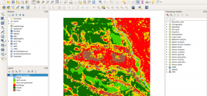
Now import the generated image in QGIS. You can change the style of the raster : in the layers panel (left side of the window), right-click on the image then select properties,and import the provided legend_style.qml file.
Import the output classification map in QGIS
Important note: We just have run the CNN in patch-based mode, meaning that the application extracts and process patches independently at regular intervals. This is costly, because the sampling strategy requires to duplicate a lot of overlapping patches, and process them independently. The TensorflowModelServe application enables to uses fully convolutional models, enabling to process seamlessly entire output images blocks... but that's also another story!
Conclusion
This tutorials has explained how to perform an image classification using a simple deep learning architecture.
The OTBTF, a remote module of the Orfeo ToolBox (OTB), has been used to process images from a user’s perspective: no coding skills were required for this tutorial. QGIS was used for visualization purposes.
We will be at IGARSS 2019 for a full day tutorial extending this short introduction, and we hope to see you there!
I am happy to announce the release of my book “Deep learning for remote sensing images with open-source software” on Taylor & Francis (https://doi.org/10.1201/9781003020851). The book extends significantly this tutorial, keeping the same format. It contains further sections to learn how to apply patch-based models, hybrid classifiers (Random Forest working on Deep learning features), Semantic segmentation, and Image restoration (Optical images gap filling from joint SAR and time series).
Bibliography
[1] R. Cresson, A Framework for Remote Sensing Images Processing Using Deep Learning Techniques. IEEE Geoscience and Remote Sensing Letters, 16(1) :25-29, 2019.
[2] Liangpei Zhang, Lefei Zhang, and Bo Du. Deep learning for remote sensing data : A technical tutorial on the state of the art. IEEE Geoscience and Remote Sensing Magazine, 4(2) :22–40, 2016.
[3] Diederik P Kingma and Jimmy Ba. Adam : A method for stochastic optimization. arXiv preprint arXiv :1412.6980, 2014.
 You can read more here.