Clouds in optical images sucks. But machine learning provides interesting methods to get rid of them! Recently, we have conducted a study for the French Space Agency to benchmark some deep learning based and deterministic approaches. This post makes an insight into our results (you can read our preprint here) and unveils Decloud, our open-source framework for Sentinel-2 images reconstruction and cloud removal.

Introduction
Well, I don’t know very much about clouds. But as a remote sensing user, all I see is how they affect the optical images: pixels in thin or thick cloud are brighter, pixels in shadows are darker. Clouds are messing with optical sensors radiometry, and we generally resort to pre-processing to deal with the polluted pixels. How can we retrieve the radiometry of an optical image impacted by clouds?
For a long time, gap-filling was used to prepare optical time-series: it interpolates the pixels in the temporal domain, using cloud masks to avoid the cloudy pixels. It works fine, is straightforward and fast. However, it relies on the cloud masks, hence depends greatly of the quality of these clouds masks. Also, it is prone to generate artifacts locally, typically when some neighboring pixels are computed with different set of dates with subtle changes in the land cover or aerosols. More recently, a plethora of deep-learning based methods have emerged, claiming SOTA results to remove clouds in optical images. Thanks to the flexibility of the convolutional neural networks, various geospatial sources have been used: coarser resolution optical images, Synthetic Aperture Radar (SAR) thanks to the Sentinel constellation, Digital Elevation Models (DEM), etc.
The existing deep-learning based methods for clouds removal or image reconstruction available in the literature are ridiculously simple, and are easy to implement. Most of the time, a convolutional neural network is trained to minimize the error between a target image (cloud-free) and the generated image. Many approaches exist: some of them use input cloud-free optical images to estimate a synthetic optical image at another date (e.g. here or here with an additional Digital Elevation Model at input), other approaches input one cloudy optical image and one SAR image and try to remove the clouds (e.g. here), other employs different/additional input sensors, etc. Some studies have started to try to model jointly the cloud generation problem and the cloud removal, but for now, with inferior results compared to real data (e.g. here). No doubt that we are just in the beginning of this fascinating research topic. Maybe in a few years, cloudy optical images will be just a distant memory?
While machine learning based approaches look promising, we must compare them with traditional approach. More importantly, we have to assess how do they perform in term of computational and technical requirements, in operational contexts?
Considered approaches and modalities
In our study, we have tried to measure how various approaches perform in terms of image quality metrics of the 10m spacing channels (Red, Green, Blue, Near infra-red) of the reconstructed image: Peak to Noise Signal Ratio (PSNR), Mean Squared Error (MSE), Structural Similarity (SSIM), Spectral Angle (SAM) were computed with a cloud-free reference image to evaluate the quality of the reconstructed image. We have focused our efforts on the following kind of approaches:
-
- (A) The traditional gap-filling: reconstruct an optical image at date t, from two optical images acquired respectively before (t-1) and after (t+1). The gap-filling does not use any SAR image, neither DEM. Also, it doesn’t use the damaged optical image at date t for the reconstructed pixels.
- (B) The deep-learning based cloud removal of one optical image using a single SAR image acquired near t. This approach, introduced in Meraner et al. (2020), uses one damaged optical image and a SAR image acquired close by, to reconstruct the missing parts of the optical image. The use of SAR image is interesting because SAR is not as sensitive as the cloud coverage as the optical image, and provide different information (Sentinel-1 VV/VH is C-Band).
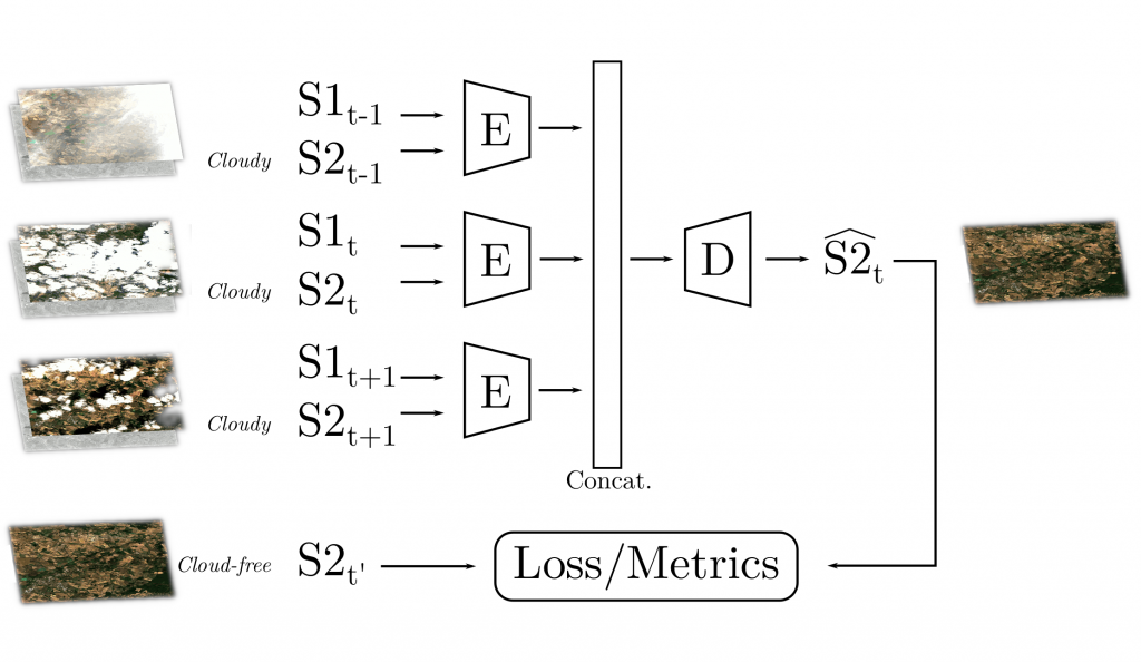
- (C) The deep-learning based cloud removal of one optical image using a single SAR image acquired near t, plus two pairs of (optical SAR) acquired respectively before (t-1) and after (t+1). This generalizes the precedent described single-date approach to multi-temporal.

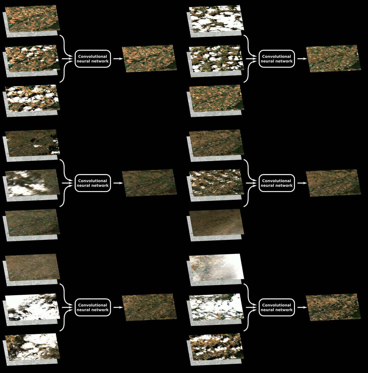
Moreover, to disentangle the benefit of the different modalities, we have conducted an ablation study on the deep nets:
-
- With optical only
- With optical + SAR
- With optical + SAR + DEM
Our results are quite interesting, showing that SAR and DEM greatly help with the cloud removal process for both (B) and (C) architectures.
Data
We have ran our experiments on every available S1 and S2 images over the Occitanie area in south of France, from january 2017 to january 2021. That represents a total of 3593 optical images over 10 tiles, and a total of 5136 SAR images in ascending orbit (in order to limit the number of SAR images, and to be able to compare our results in other regions of the world, we deliberately chose to keep only the ascending orbits of the Sentinel-1 images: indeed in most places in the world, only a single orbit is available).
One challenge was to create datasets that enable to train the deep learning based approaches, and more importantly, to compare all approaches, fitting all benchmarked models validity domains. For this, we have developed a sample generation framework that uses an R-Tree to index the cloud percentage, nearest SAR image to optical, acquisition date, of every available patches in our study sites.
Using our framework, we have crafted datasets enabling the comparison of approaches having different modalities and requirements/constraints at input. It was trivial to compare approaches (B) and (C) since we can use the (optical, SAR) pair at date t, from the dataset enabling the testing of (B), i.e. which is composed of pairs of images at dates t-1, t and t+1 (only the pairs at t is used for approach C). However, to compare (A) and (B), it was a bit more complicated. Indeed, we had to find cloud-free images at t-1 and t+1, but also, in order to mimic the operational situation, we wanted the optical image at t to be 100% cloudy (typically, we would have used gap-filling in this situation in real life). We called acquisitions layout the way images must be acquired in a particular situation: e.g. between [0%, 100%] cloudy at date t, with a SAR image acquired close, and a reference cloud-free optical image acquired less than 10 days from the cloudy image (we give a few examples later below). Except for the gap-filling, which doesn’t require training, this reference image (or target image) is used from the training dataset to optimize the network, and from the test dataset, it is used to compute the evaluation metrics (PSRN, MSE, SSIM, SAM). Talking about datasets splits: we have selected ROIs in the geographical domain to avoid any patch overlap from the training and test groups, to ensure that we don’t measure any over-fitting of the networks.
The following figure explains how acquisitions layouts work:

Specifically, here is the acquisitions layout that we used to train (B). This architecture is very simple: it inputs one SAR image (S1t) and a potentially cloudy optical image (S2t), and outputs the de-clouded optical image (Ŝ2t). The setting to train (B) is very basic: we just need one (S1t, S2t) pair with S2t possibly cloudy, and the dates of the SAR and optical being close, and a target cloud-free S2target acquired close to the S2t image. The model is trained minimizing the average absolute error between Ŝ2t and S2target.

And it is the same thing for the (C) network, with additional SAR and optical images at t-1 and t+1:
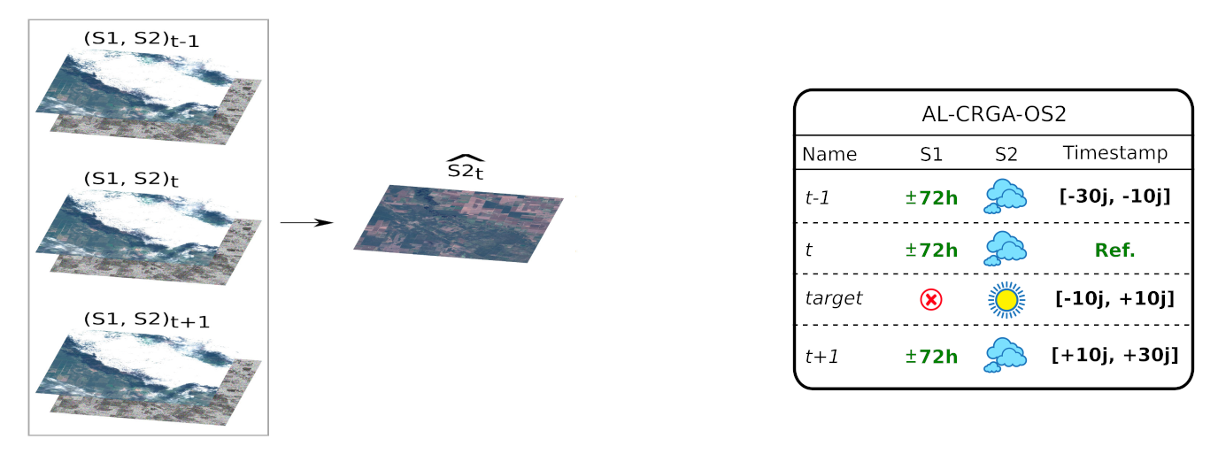
In all acquisitions layouts, the values for time ranges and optical-to-SAR maximum gap were chosen regarding the orbits of Sentinel-1 and Sentinel-2 over our study site. Since Sentinel-1 and Sentinel-2 swathes do not overlap in the same fashion everywhere in the world, these parameters might not be suited for another area.
Now, to compare gap-filling with deep-learning based approaches, we had to create other datasets (“OS2GFa” and “OS2GFb”) for which all models validity domains fit. The following figure illustrates how this can be accomplished, setting wise time ranges with the adequate cloud cover ranges for t-1, t and t+1 .

Benchmarks
Well, the goal here is not to rewrite our paper, so we will be short! You can take a look on the Decloud source code to see how it is done, and read the paper here for more specifics.
In short, first we have pre-processed our S1 and S2 images using the CNES HAL cluster and datalake. Thanks to the S1Tiling remote module of the Orfeo ToolBox, the download and the calibration of the S1 image are completely automated, saving us a great deal of pain. We used the S2 images from the Theia land data center, in Level 2A processed with the MAJA software since the clouds masks are included in the products (we recall that we used the cloud masks only as metadata per patch, for the estimated cloud coverage percentage). After that, we have generated our datasets from the carefully crafted acquisitions layouts. Then, we have trained our deep nets over their respective training datasets, to minimize the l1 distance between the generated image, and the reference image. We have run all experiments on the Jean-Zay computer at IDRIS. Finally, we have computed the image quality metrics of the reconstructed images over various test datasets (we recall that each one have a null intersection with the training dataset, in the geographical domain).
The (B) network was implemented from its original formulation. Although their paper is amazing and inspiring, their network is greedy in terms of computational resources. So much, that we believe it is not applicable regarding the extremely long processing time required. We hence have modified their original implementation, reducing the processing time with a factor of (roughly) 30x, with the same outcomes in terms of image quality metrics. We gave a few details in our paper: in short we have replaced their ResNet-based bottleneck with a U-Net, which have several benefits e.g. used sources with different spatial resolutions in input and output. The ablation study was performed on our version of (B), since we could have run more experiments in reasonable time.

The (C) network generalizes (B): same U-Net backbone, shared encoders, and the decoder applied over the stacked features maps of the encoder. Take a look in our code!
Results
Comparison of single-date based approaches (b)
We first have compared the original network based on a ResNet backbone, with our modified version with a U-Net backbone. The first shocking information is that the modified version is sometimes like 30-40x faster. Instead of days of training, it’s now just hours. Same thing for the inference. This can be explained because the ResNet performs over features at 10m spatial resolution, unlike the U-Net which performs convolutions on downsampled features. The memory footprint is reduced, and less operations are required since convolutions are performed on features maps of smaller size. Another advantage of the U-Net is that it can deal natively with sources of different resolutions, e.g. a DEM or 20m spacing bands can be concatenated after the first downsampling step in the encoder, and the output 20m spacing bands can be retrieved after the second last upsampled convolutions of the decoder. Indeed, in the original implementation, the ResNet processes everything at the highest resolution, hence any input has to be resampled at 10m (e.g. the 20m spacing bands), same for the outputs… not very computationally efficient!
The results show very little difference in terms of image quality metrics, between the U-Net and the ResNet based networks. We believe that the SSIM is slightly higher with the ResNet based approach since less details are lost because the network performs the convolutions without any downsampling, or because of the residual correction (this has to be investigated further). The results show how the SAR and the DEM help reconstructing the cloudy image, especially in terms of radiometric fidelity (PSNR, MSE, SAM):

We can appreciate visually the benefit of the different modalities, in the figure below:
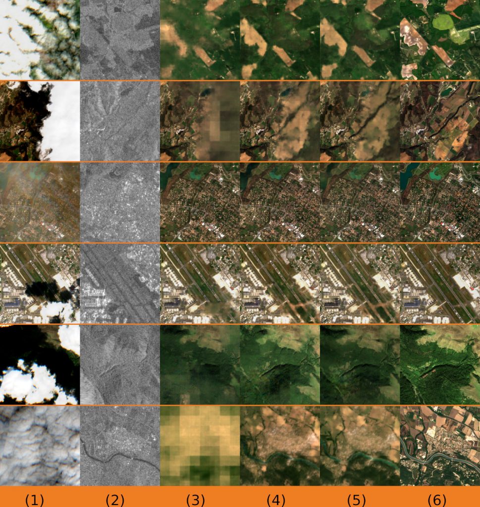
As you can see, when no information available, the network cannot do magic stuff, and fails to retrieve something good. Anyway, I am still amazed how it is able to catch the average radiometry from a mixture of thick cloudy pixels… To the question “how does SAR and DEM help?”, we can only conjecture. But experimental results show how these sources benefit to the cloud removal process.
Deep-learning based, single-date vs multitemporal
Ok, we all know that it is not a fair fight! Anyway. Here we just compare (B) and (C) over the test dataset of (C), using only the images at central date t for (B).
With no surprise, the multi-temporal helps a lot. Even without SAR image it still outperforms the single-date based model. Again, we can observe that the SAR and DEM inputs helps the network toward a better reconstruction of the optical image.

The following illustration shows how the SAR and the DEM help to retrieve the missing contents in the polluted optical image:
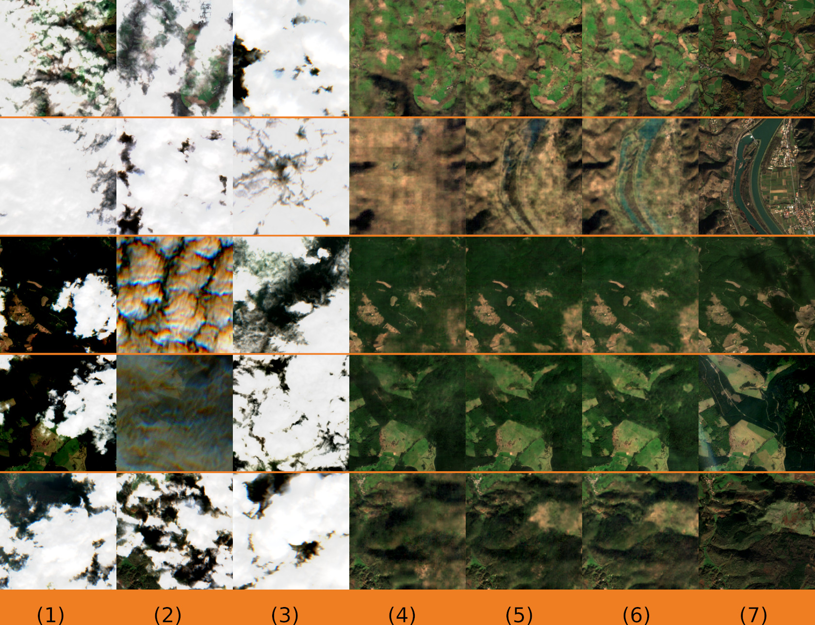
As you can see, sometimes the reconstructed image has less clouds than the reference image! (4th row)
Comparison of All approaches
Now we want to compare all approaches together. In operational situation, we will mostly use gap-filling to retrieve one pixels which is occluded by clouds. From here, we have created an acquisitions layout where the optical image at date t is completely cloudy, and images at t-1 and t+1 are completely cloud-free, because gap-filling also can only work with these two available cloud-free optical images.
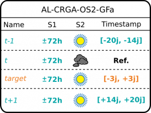
A small detail: the gap-filling is performed to reconstruct the image at date target instead of t, to remove this small temporal bias.
Now, we measure how perform (B) and (C) in this setup, which corresponds to a situation where the gap-filling should be a bit advantaged.
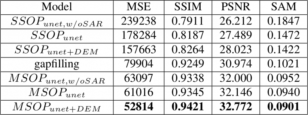
We can notice that the gap-filling outperforms the single-date based (B) approach. Not doubt that in this situation, available cloud-free images helps more that a SAR image! But it is completely outperformed by the multi-temporal deep-learning approaches of (C). Even without SAR images, the reconstruction is better. Note also that this operational situation is not nominal for the (C) approach, which can be applied over cloudy input images, unlike the gap-filling.
Below are a few screenshots over the test patches:
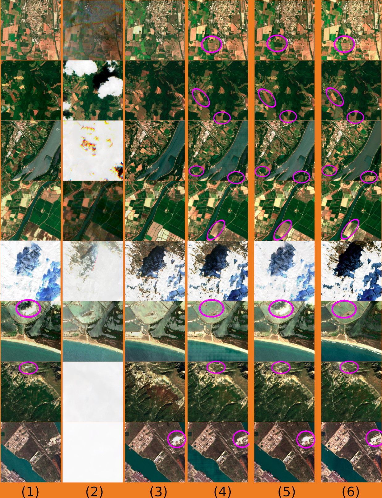
You can observe that cloud masks are not always perfect, and lead to artifacts in the images generated using the gap-filling (caused by clouds in the input images, that the masks have missed). Gap-filling typically uses per-pixel clouds masks, it is then very dependent of their quality. On the contrary, the convolutional deep nets are very good in removing the clouds, even though they have been trained from datasets generated using the cloud coverage information (but not the per-pixel oriented cloud mask). Another interesting thing we can observe is the ability of the deep learning based approaches to better reconstruct the sudden changes in time series, possibly due to the use of the available pixels of the optical image at date t, even if cloudy or in the cloud shadows, and the SAR image at t.
We have visually remarked a small drawback of SAR+optical convolutional neural networks over water areas, with small artifacts (row 6). We believe that it’s hard for the network to train on this target, since its surface is changing rapidly (swell, wind, …) and because the SAR backscatter is very sensitive to the water surface roughness.
Computational requirements
Training
We have trained all our networks from approximately 600k training samples, on quad-GPU (NVIDIA V100 with 32Gb RAM). Our networks have less than 30k parameters.
The slowest network is the original (B), trained in 30-40 days. All other networks were trained in less than 42 hours (models C) and 20 hours (models B, modified with U-Net backbone).
Full scene inference
Since our goal was not just to generate nice RGB patches for the reviewers, we have developed pipelines to process seamlessly entire S2 images end-to-end with OTB applications and the OTBTF remote module. The time required to process one entire S2 image with the (C) network is approximately 2 minutes with an old NVIDIA GTX1080Ti. For the (B) network I don’t know but it must be something like 1-2 minutes for an entire Sentinel-2 image.

Conclusion
We have compared single date and multitemporal convolutional networks with the traditional gap-filling, showing the benefits of the SAR and DEM inputs for the optical image reconstruction.
Also, we have shown that, even if the primary design of the multitemporal convolutional network is not focused on image interpolation in temporal domain, it leads to better results than the gap-filling. We also showed that single date based networks cannot be substituted to gap-filling for the estimation of a completely cloudy image at date t. Single date networks are great over thin clouds, but we have noticed that they fail to retrieve the image details under thick clouds, and lead to blurry images.
However, we should interpret our results carefully regarding the ancillary data available for cloud coverage characterization, since our cloud coverage information per patch depends from it. In addition, we lead our study over a small area that do not represents the various atmospheric conditions all over the earth!
Many other things could be investigated in future studies. For instance, could the geometric parameters of SAR, or physical based SAR pre-processing, help? Is there better loss functions to train the networks? Which architectures are better suited to time series? etc.
Final words
Thanks to the flexibility of the deep nets, it is easy to tailor (nearly) anything to a particular problem, and we can mix the different inputs and outputs with an unprecedented ease (We still have to think a bit though!). For operational use, the preparation of training data and the required processing time are crucial points. Regarding the specific problem of optical image clouds removal, no doubt that deep nets will help to deliver more exploitable data in the future!
Take a look in our code. It is based on Orfeo ToolBox with the OTBTF remote module and the PyOtb extension, GDAL and TensorFlow. We have a pre-trained model for the south of France, and another for the west of Burkina Faso: try them! Don’t forget to raise issues, do not hesitate to contribute!
Happy deep learning.
